
PhD Thesis — Optimal Sampling for State Estimation and Control
I started working on my Ph.D. thesis in 2017 with Prof. Raphaël Jungers and Prof. Benoit Macq. My Ph.D. thesis was motivated by an applied problem in proton therapy, a cancer treatment method that targets tumors with a proton beamline. The success of this approach relies on precise knowledge of the tumor’s position, which becomes particularly challenging for mobile tumors, such as lung tumors, that move with the patient’s breathing. One approach to address this challenge is to use X-ray images of the patient’s chest to measure the tumor’s position. However, X-ray imaging exposes both the tumor and healthy tissue to radiation, limiting the number of images that can be safely taken.
My thesis addresses the problem of determining the optimal timing for X-ray acquisitions, within a limited budget, to maximize the accuracy of the tumor tracking.
From a more abstract perspective, this problem can be formulated as optimizing the measurement times to obtain the best state estimation of a dynamical system. I studied this problem under different assumptions: linear vs. nonlinear dynamics; expected vs. worst-case error.
Despite the practical motivation behind my thesis, my research has been primarily (though not exclusively) theoretical, with a strong focus on its potential for real-world, safety-critical applications.
Linear and Gaussian dynamics: Optimal intermittent Kalman filter
In a first phase of my thesis, I focused on the case of a linear system subject to Gaussian process and measurement noises, fitting the Kalman filter formalism. My goal is to select the measurement times in order to minimize the cumulated expected mean squared error.
This research led to the following publication:
- Antoine Aspeel, Axel Legay, Raphaël M Jungers, and Benoit Macq. Optimal measurement budget allocation for Kalman prediction over a finite time horizon by genetic algorithms. In EURASIP Journal on Advances in Signal Processing, 2021.
The linear system we are considering can be written
\[\begin{aligned} x_{t+1} &= Ax_t + w_t \\ y_t &= \begin{cases} Cx_t + v_t & \text{if } \sigma_t = 1 \\ \emptyset & \text{else.} \end{cases} \end{aligned}\]where $x_t$ is the state, $y_t$ is the measurement, $w_t$ and $v_t$ are process and measurement noises. They are independent and follow a Gaussian distribution. The quantity $\sigma_t\in$ {0,1} is a binary variable describing when a measurement is acquired. This dynamics is considered over a finite time horizon $t=0,\dots,T$, and a budget of at most $N$ measurements is allowed, i.e., $ \sum_{t=0}^T\sigma_t\leq N$.
In this research, my goal is to design the measurement times $(\sigma_t)_{t=0}^T$ in order to minimize the cumulated expected mean squared estimation error
\[\sum_{t=0}^T \mathbb{E}[\|x_t-\hat{x}_t\|^2_2],\]where
\[\hat{x}_t=\mathbb{E}[x_t| y_0,\dots,y_t]\]is the minimum mean squared error estimate. For a given sequence of measurement times $(\sigma_t)_{t=0}^T$, the estimate $\hat{x}_t$ is given by the Kalman filter (the correction step of the Kalman filter is skipped when $\sigma_t=0$ and no measurement is available).
Time- vs. self-triggered measurements: In order to make the estimation error as small as possible, the decision $\sigma_t$ of measuring at time $t$ should depend on all the available information at that time, including the previous measurements $y_0,\dots,y_{t-1}$. Formally, this can be written
\[\sigma_t=\pi_t(\sigma_0,\dots,\sigma_{t-1};y_0,\dots,y_{t-1}),\]where $\pi_t$ is a policy function. In that case, the measurement-times selection mechanism is called self-triggered.
In contrast, if the measurement times $\sigma_t$ are selected a priori, independently of the measurements, the measurement-times selection is called time-triggered. In general, time-triggered mechanisms are easier to implement, but self-triggered mechanisms give better performance.
Designing self-triggered mechanisms poses the following computational challenges:
- Challenge: The optimization variables are the policy functions
that decide if a measurement is necessary at time $t$ based on the previously acquired measurements $y_0,\dots,y_{t-1}$. Since functions are infinite dimensional objects, this makes the problem infinite-dimensional and therefore seemingly intractable.
Solution: A key finding of this part of my research is that the optimal policies do not depend on the measurements. Consequently, one can optimize directly over the measurement times $(\sigma_t)_{t=0}^T$ making the problem finite-dimensional. In other words, we showed that the optimal self-triggered and time-triggered mechanisms are equivalent. In addition, the measurement times can be selected offline (i.e., before the beginning of the tracking at time $t=0$) without loss of optimality.
- Challenge: Despite being finite-dimensional, optimizing over the measurement times $(\sigma_t)_{t=0}^T$ is an intractable combinatorial optimization problem.
Solution: We proposed an efficient genetic algorithm specifically tailored to this optimization problem.
Using a duality argument, our method can be applied to control a linear system subject to an actuation budget while minimizing a LQR cost.
Application to tumor tracking and industrial collaboration
Throughout my Ph.D., I had the privilege of collaborating with IBA (Ion Beam Applications), the world-leading company in proton therapy. This partnership allowed me to bridge the gap between theory and practice by applying the methods I developed to tumor tracking using real medical data.
- Challenge: Proton therapy involves targeting tumors with an ionizing proton beam, requiring precise knowledge of the tumor’s position to minimize irradiation of healthy tissues. This precision is especially challenging for lung tumors, which move with the patient’s breathing. A common clinical approach involves acquiring X-ray images of the chest to determine the tumor’s position. However, the use of X-rays must be limited to reduce radiation exposure to healthy tissues.
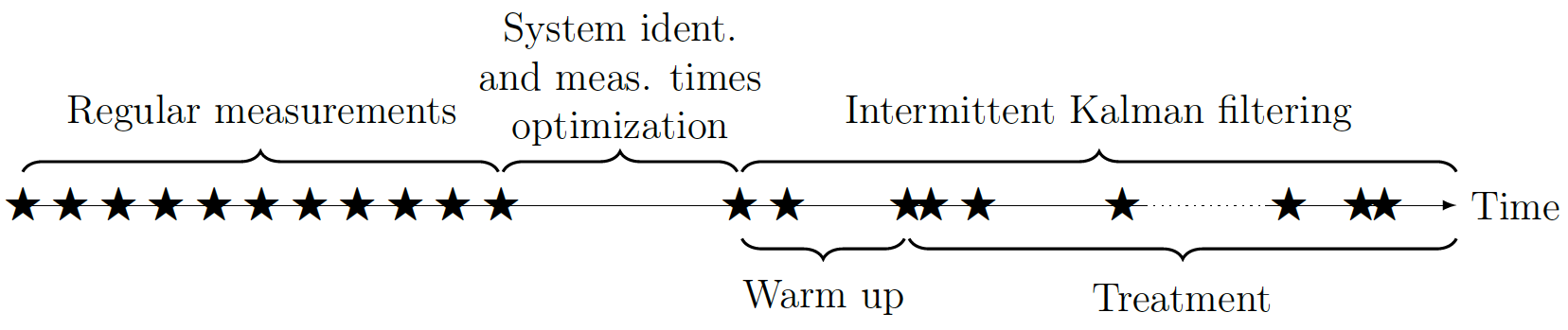
Solution: We proposed the following clinical workflow for tracking lung tumors using time-triggered X-ray acquisitions (see figure below): Before treatment, regular X-ray images of the patient’s chest are acquired. Then, a system identification method is used to construct a linear model of the tumor’s motion. Using this model, our optimal intermittent Kalman filter determines future X-ray acquisition times and tracks the tumor during treatment.
Using real patient data, we demonstrated that optimizing X-ray acquisition times with our intermittent Kalman filter significantly improves tumor tracking, thereby enhancing the effectiveness of the treatment.
This more applied contribution resulted in the following medical publication:
- Antoine Aspeel, Damien Dasnoy, Raphaël M Jungers, and Benoit Macq. Optimal intermittent measurements for tumor tracking in X-ray guided radiotherapy. In Medical Imaging 2019: Image-Guided Procedures, Robotic Interventions, and Modeling. International Society for Optics and Photonics, 2019.
Nonlinear and non-Gaussian dynamics: Optimal intermittent particle filter
In a second phase of my Ph.D., I considered the case of nonlinear dynamical systems subject to non-Gaussian noise. My work resulted in the following publications:
Antoine Aspeel, Amaury Gouverneur, Raphaël M Jungers, and Benoit Macq. Optimal measurement budget allocation for particle filtering. In 27th IEEE International Conference on Image Processing, 2020.
Antoine Aspeel, Amaury Gouverneur, Raphaël M Jungers, and Benoit Macq. Optimal intermittent particle filter. IEEE Transactions on Signal Processing, 2022.
In that case, the optimal policy for the measurement times is not independent of the measurements, i.e., time- and self-triggered measurement mechanisms give different solutions. Therefore, we developed a time-triggered and a self-triggered method to optimize the measurement times of a particle filter.
Time-triggered particle filter
We started by considering the problem of finding the best time-triggered measurement times, i.e., the measurement times $(\sigma_t)_{t=0}^T$ must be selected offline and are not allowed to depend on the measurements $y_0,\dots,y_T$.
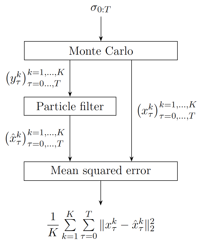
- Challenge: Since the dynamics are nonlinear and stochastic, estimating the cumulated expected mean squared error for a specific sequence of measurement times is challenging.
Solution: We developed a Monte Carlo method that simulates the dynamics to estimate the cumulated estimation error (see figure below).
Self-triggered particle filter
To design a self-triggered particle filter, we used a receding horizon approach. First, all measurement times are selected offline using our time-triggered particle filter. Then, only the first measurement is acquired, and the remaining measurement times are re-optimized by taking into account the already received measurements. This process is repeated until the measurement budget $N$ is reached.
- Challenge: Receding horizon approaches require online (i.e., real-time) computations, which can become infeasible in practice due to computational limitations.
Solution: To mitigate the computational burden, we employed warm-start techniques, parallelization, and problem-specific decomposition strategies, achieving a significant reduction in computation time.
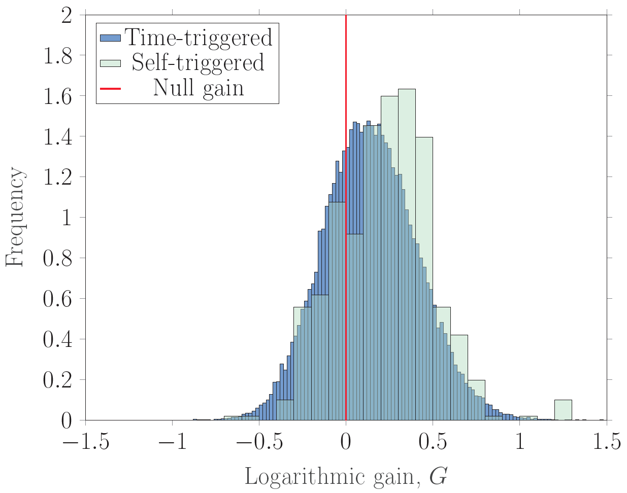
Overall, both of our methods have their merits: the time-triggered particle filter is easier to implement because it avoids online computations, while the self-triggered particle filter offers provably better performance. In addition, both methods outperform filtering with regularly spaced measurements (see figure below).
Beyond mean squared error: Optimal sampling for worst-case control
This part of my research was published in
- Antoine Aspeel, Kwesi Rutledge, Raphaël M Jungers, Benoit Macq, and Necmiye Ozay. Optimal control for linear networked control systems with information transmission constraints. In The 60th IEEE International Conference on Decision and Control, 2021.
We considered a linear control system subject to bounded disturbances together with a linear controller with memory, i.e.,
\[u_t = \sum_{\tau \leq t} K_{(t,\tau)} y_\tau,\]where the gains $K_{(t,\tau)}$ are design variables. Our objective was to co-design:
- the controller gains $K_{(t,\tau)}$,
- the measurement times $\sigma_t^{\text{meas.}}$,
- the control times $\sigma_t^{\text{control}}$,
while satisfying two types of constraints:
- a safety constraint ensuring that the state remains inside a prescribed safe region for any realization of the disturbances,
- a budget constraint on the use of sensors and actuators.
Safety
The safety constraint is not convex with respect to the controller gains $K_{(t,\tau)}$. However, using the Youla parameterization allows one to rewrite the constraint linearly in terms of the Youla parameter (assuming safety and noise sets are polytopes).
Budget
The budget constraints can be written as
\[\sum_{t=0}^T \sigma_t^{\text{meas./control}} \leq N^{\text{meas./control}}.\]For the controller structure above, the budget constraints on sensors and actuators can be handled using linear indicator constraints on the controller gains:
\[\begin{aligned} \sigma_\tau^{\text{meas.}} = 0 &\Rightarrow \left( K_{(t,\tau)} = 0 \text{ for all } t \right), \\ \sigma_t^{\text{control}} = 0 &\Rightarrow \left( K_{(t,\tau)} = 0 \text{ for all } \tau \right). \end{aligned}\]The first constraint ensures that if a measurement is unavailable at time $\tau$, it cannot be used by the controller. The second constraint guarantees that $u_t = 0$ whenever $\sigma_t^{\text{control}} = 0$.
- Challenge: Solving the problem directly in terms of the controller gains leads to a non-convex safety constraint. Conversely, solving the problem in terms of the Youla parameter may render the indicator constraints non-convex.
Solution: We proved that, despite the nonlinearity of the Youla parameterization, the linearity of the indicator constraints is preserved through this specific nonlinear change of variables. This result allows the problem to be reformulated as a mixed-integer linear program (MILP), instead of a mixed-integer non-convex program, yielding considerable computational benefits.